Photon extractor

The photon extractor challenge is based on “Inverse-designed photon extractors for optically addressable defect qubits” by Chakravarthi et al.; it involves optimizing a GaP patterned layer on diamond substrate above an implanted nitrogen vacancy defect. An oxide hard mask used to pattern the GaP is left in place after the etch.

The goal of the optimization is to maximize extraction of 637 nm emission, i.e. to maximize the power coupled from the defect to the ambient above the extractor. Such a device device could be useful for quantum information processing applications.

Simulating an existing design

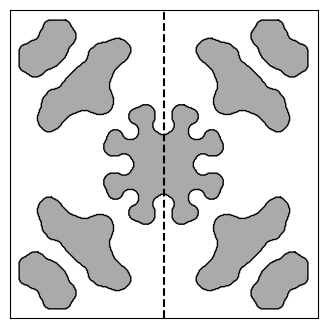
We’ll begin by loading, visualizing, and simulating the design reported in the reference. Later, we’ll plot an x-z cross section of fields in the extractor, which is indicated below with the dashed black line.

import matplotlib.pyplot as plt
import numpy as onp
from skimage import measure

design = onp.genfromtxt(
    "../../../reference_designs/photon_extractor/device1.csv",
    delimiter=",",
)

plt.figure(figsize=(4, 4))
ax = plt.subplot(111)
im = ax.imshow(1 - design.T, cmap="gray")
im.set_clim([-2, 1])
contours = measure.find_contours(design.T)
for c in contours:
    plt.plot(c[:, 1], c[:, 0], "k", lw=1)
ax.set_xticks([])
ax.set_yticks([])

midpoint = design.shape[0] / 2
ax.plot([midpoint, midpoint], [0, design.shape[0]], "k--")
ax.set_xlim([120, design.shape[1] - 120])
_ = ax.set_ylim([120, design.shape[0] - 120])

We will use the Challenge object returned by challenges.photon_extractor to carry out the simulation.

from invrs_gym import challenges

challenge = challenges.photon_extractor()

To simulate our photon extractor, we need to create a totypes.types.Density2DArray object that has this padded design as its array attribute. We obtain dummy parameters and then overwrite them with our design.

import dataclasses
import jax

dummy_params = challenge.component.init(jax.random.PRNGKey(0))
params = dataclasses.replace(dummy_params, array=design)

We are now ready to simulate the photon extractor, using the component.response method. By default, this will not compute the fields emitted by the source (for improved performance), but we will do so here for visualization purposes.

response, aux = challenge.component.response(params, compute_fields=True)

1.0

1.38

In this challenge, we care about the enhancement in flux compared to a bare substrate. This is included in the challenge metrics, for x-, y-, and z-oriented dipoles.

metrics = challenge.metrics(response, params=params, aux=aux)
for i, orientation in enumerate(["x", "y", "z"]):
    print(
        f"Flux enhancement for {orientation} dipole is "
        f"{metrics['enhancement_flux_per_dipole'][i]:.2f}"
    )

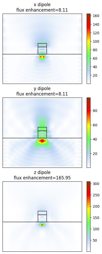
Flux enhancement for x dipole is 7.61
Flux enhancement for y dipole is 7.92
Flux enhancement for z dipole is 146.94

The values are similar to those reported by Chakravarthi et al.

Now let’s visualize the fields; these are for an xz slice, and are computed for each of the dipole orientations. Plot the field magnitude for each dipole orientation with the structure overlaid.

from skimage import measure

x, y, z = aux["field_coordinates"]
ex, ey, ez = aux["efield"]

assert ex.ndim == 3 and ex.shape[-1] == 3
field_magnitude = onp.sqrt(onp.abs(ex) ** 2 + onp.abs(ey) ** 2 + onp.abs(ez) ** 2)
maxval = onp.amax(field_magnitude)


# Define a function that will plot the fields and overlay the structure.
def plot_field_and_structure(ax, field, title):
    # Plot the field.
    xplot, zplot = onp.meshgrid(x, z, indexing="ij")
    ax.pcolormesh(xplot, zplot, field, cmap="magma")

    # Overlay the structure.
    spec = challenge.component.spec

    z0 = spec.thickness_ambient
    z1 = z0 + spec.thickness_oxide
    z2 = z1 + spec.thickness_extractor

    # Plot line at the top of the substrate.
    ax.plot([0, onp.amax(x)], [z2, z2], "w", lw=1)

    density_plot = params.array
    density_plot_slice = density_plot[:, density_plot.shape[1] // 2, onp.newaxis]
    contours = measure.find_contours(onp.tile(density_plot_slice, (1, 2)))
    for c1, c2 in zip(contours[::2], contours[1::2]):
        zc = onp.concatenate([c1[:, 1], c2[:, 1], [0]])
        xc = onp.concatenate([c1[:, 0], c2[:, 0], [c1[0, 0]]]) + 0.5
        xc = xc * (x[1] - x[0]) + x[0]
        zcp = onp.where(zc == 0, z0, z1)
        ax.plot(xc, zcp, "w", lw=1)  # Oxide
        zcp = onp.where(zc == 0, z1, z2)
        ax.plot(xc, zcp, "w", lw=1)  # GaP

    ax.set_xlim([0, onp.amax(x)])
    ax.set_ylim([onp.amax(z), 0])
    ax.axis("equal")
    ax.axis(False)
    ax.set_title(title)


plt.figure(figsize=(4, 12))
plot_field_and_structure(
    plt.subplot(311),
    field_magnitude[:, :, 0],
    title=f"x dipole; flux enhancement={metrics['enhancement_flux_per_dipole'][0]:.2f}",
)
plot_field_and_structure(
    plt.subplot(312),
    field_magnitude[:, :, 1],
    title=f"y dipole; flux enhancement={metrics['enhancement_flux_per_dipole'][1]:.2f}",
)
plot_field_and_structure(
    plt.subplot(313),
    field_magnitude[:, :, 2],
    title=f"z dipole; flux enhancement={metrics['enhancement_flux_per_dipole'][2]:.2f}",
)

The resulting figures are a bit asymmetric, but this is not entirely unexpected since the reference design lacks symmetry.