Metalens

The metalens challenge entails designing a one-dimensional metalens that focuses blue, green, and red light (450 nm, 550 nm, and 650 nm) to the same point in space. This problem was studied in “Validation and characterization of algorithms and software for photonics inverse design” by Chen et al.; the associated photonics-opt-testbed repo contains several example designs.

Simulating an existing design

We’ll begin by loading, visualizing, and simulating a design from the photonics-opt-testbed repo.

import matplotlib.pyplot as plt
import numpy as onp
from skimage import measure

design = onp.genfromtxt(
    "../../../reference_designs/metalens/Rasmus70nm.csv",
    delimiter=",",
)

plt.figure(figsize=(8, 2))
ax = plt.subplot(111)
im = ax.imshow(1 - design.T, cmap="gray")
im.set_clim([-2, 1])
contours = measure.find_contours(design.T)
for c in contours:
    plt.plot(c[:, 1], c[:, 0], "k", lw=1)
ax.set_xticks([])
ax.set_yticks([])
_ = ax.set_xlim(100, 700)

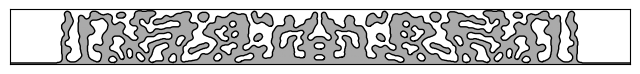
As in other examples, we will use the metalens challenge to simulate this design. However, we need to configure the challenge so that the design region size and grid spacing precisely match the reference. All of these physical characteristics are stored in a MetalensSpec object. Modify the defaults to match our design, pad design so that it has the shape required by the challenge, and then create the challenge object.

import dataclasses
from invrs_gym import challenges
from invrs_gym.challenges.metalens import challenge as metalens_challenge

# By default the simulation does not use PML, but we include it here for visuals.
grid_spacing = metalens_challenge.METALENS_SPEC.grid_spacing
spec = dataclasses.replace(
    metalens_challenge.METALENS_SPEC,
    width_pml=0.5,
    pml_lens_offset=2.5,
    pml_source_offset=2.0,
    grid_spacing=grid_spacing,
)

challenge = challenges.metalens(spec=spec)

To simulate our metalens design, we need to create a totypes.types.Density2DArray object that has this design as its array attribute. We obtain dummy parameters and then overwrite them with our design.

import jax

dummy_params = challenge.component.init(jax.random.PRNGKey(0))
params = dataclasses.replace(
    dummy_params, array=design, fixed_solid=None, fixed_void=None
)

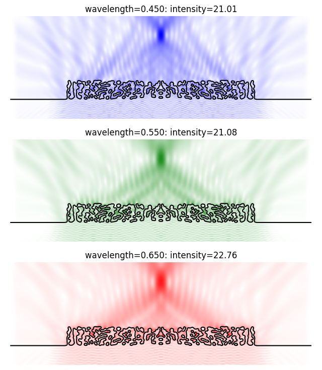
We are now ready to simulate the metalens, using the component.response method. By default, this will not compute the fields passing through the metalens (for improved performance), but we will do so here for visualization purposes.

response, aux = challenge.component.response(params, compute_fields=True)

The response includes the intensity at the focus for each of the three wavelengths.

for wvl, enhancement in zip(response.wavelength, response.enhancement_ex):
    print(f"Intensity for wavelength={wvl:.3f} is {enhancement:.2f}")

Intensity for wavelength=0.450 is 20.96
Intensity for wavelength=0.550 is 21.05
Intensity for wavelength=0.650 is 22.72

These values are close to those reported in the photonics-opt-testbed repo, indicating that our simulation is well-converged. Next, let’s visualize the fields. Since we have specified compute_fields=True, in the fields are included in the aux dictionary.

from skimage import measure

ex, ey, ez = aux["efield"]
x, _, z = aux["field_coordinates"]
xplot, zplot = onp.meshgrid(x[0, :, 0], z, indexing="ij")

abs_field = onp.sqrt(onp.abs(ex) ** 2 + onp.abs(ey) ** 2 + onp.abs(ez) ** 2)

plt.figure(figsize=(8, 9))
for i, color in enumerate(["b", "g", "r"]):
    cmap = plt.cm.colors.LinearSegmentedColormap.from_list("b", ["w", color], N=256)

    ax = plt.subplot(3, 1, i + 1)
    im = ax.pcolormesh(xplot, zplot, abs_field[i, :, 0, :, 0], cmap=cmap)
    maxval = onp.amax(abs_field[i, :, 0, :])
    im.set_clim([0, maxval])
    ax.axis("equal")

    contours = measure.find_contours(onp.asarray(params.array))
    for c in contours:
        x = c[:, 0] * spec.grid_spacing
        z = c[:, 1] * spec.grid_spacing + spec.focus_offset + spec.thickness_ambient
        ax.plot(x, z, "k")

    ax.set_xlim([onp.amin(xplot), onp.amax(xplot)])
    ax.set_ylim([onp.amax(zplot), onp.amin(zplot)])
    ax.axis(False)

    ax.set_title(
        f"wavelength={response.wavelength[i]:.3f}: intensity={response.enhancement_ex[i]:.2f}"
    )

Performance versus length scale

Next, we will compute the performance of the reference devices and measure their length scale using the imageruler package.

import glob
import imageruler

results = {"rasmus": [], "mo": []}
challenge = metalens_challenge.metalens()
dummy_params = challenge.component.init(jax.random.PRNGKey(0))

for fname in glob.glob("../../../reference_designs/metalens/*.csv"):
    design = onp.genfromtxt(fname, delimiter=",")
    params = dataclasses.replace(
        dummy_params, array=design, fixed_solid=None, fixed_void=None
    )

    response, aux = challenge.component.response(params)

    # Compute the length scale in nanometers for the binary design.
    length_scale = (
        onp.amin(imageruler.minimum_length_scale(design > 0.5)) * grid_spacing * 1000
    )

    if "Mo" in fname:
        key = "mo"
    elif "Rasmus" in fname:
        key = "rasmus"

    results[key].append(
        {"response": response, "length_scale": length_scale, "aux": aux}
    )

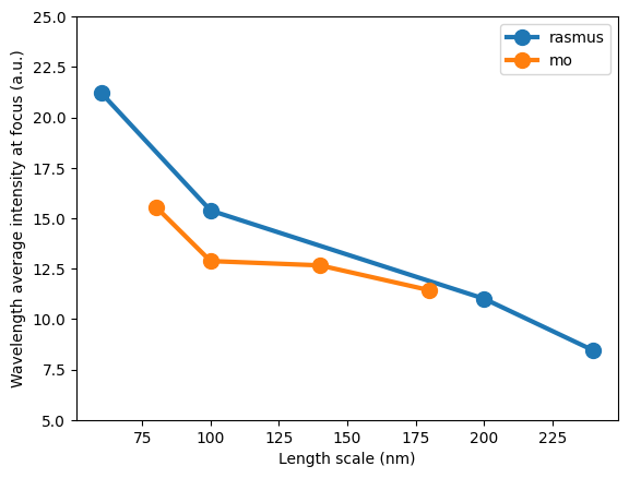
Plotting, we see results very similar to those of figure 3 of “Validation and characterization of algorithms and software for photonics inverse design” by Chen et al.

Differences are explained by updates to the imageruler algorithm and the fact that we are using a different simulation algorithm to model the metalenses. Also, the Rasmus-generated designs have been resampled to have 20 nm grid spacing (originally 10 nm) as expected by the metalens challenge.

ax = plt.subplot(111)

for key, result in results.items():
    enhancement = onp.asarray([onp.mean(r["response"].enhancement_ex) for r in result])
    length_scale = onp.asarray([onp.amin(r["length_scale"]) for r in result])
    order = onp.argsort(length_scale)
    ax.plot(length_scale[order], enhancement[order], "o-", lw=3, ms=10, label=key)

ax.set_xlabel("Length scale (nm)")
ax.set_ylabel("Wavelength average intensity at focus (a.u.)")
ax.set_ylim((5, 25))
_ = plt.legend()