Ceviche challenges

The ceviche challenges are based on “Inverse design of photonic devices with strict foundry fabrication constraints” by M. F. Schubert et al., and the associated github repo. These use the ceviche simulation engine to solve Maxwell’s equations in two dimensions, and are therefore nonphysical and serve primarily as a vehicle for evaluating optimization schemes.

The challenges include a mode converter, beam splitter, waveguide bend, and wavelength demultiplexer, with a “normal” and “lightweight” version of each. Lightweight versions have lower simulation resolution and are faster to evaluate.

In this notebook we’ll focus on the mode converter challenge—simulating an existing design, and showing how to set up an optimization problem that will give us a new mode converter. The mode converter was also studied in “Validation and characterization of algorithms and software for photonics inverse design” by Chen et al.; the associated photonics-opt-testbed repo contains several example designs.

Simulating an existing design

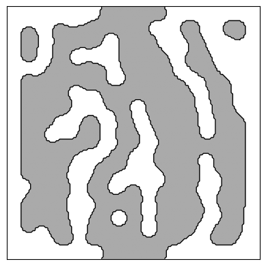
We’ll begin by loading, visualizing, and simulating one design from the photonics-opt-testbed repo.

import matplotlib.pyplot as plt
import numpy as onp
from skimage import measure

design = onp.genfromtxt(
    "../../../reference_designs/ceviche/mode_converter/converter_generator_circle_10_x47530832_w19_s483.csv",
    delimiter=",",
)

ax = plt.subplot(111)
ax.set_xticks([])
ax.set_yticks([])
im = ax.imshow(1 - design, cmap="gray")
im.set_clim([-2, 1])
contours = measure.find_contours(design)
for c in contours:
    plt.plot(c[:, 1], c[:, 0], "k", lw=1)

Now, we’ll create the ceviche_mode_converter challenge. Since we won’t be optimizing just yet, we don’t actually need the challenge itself, but rather it’s component attribute. As stated in the readme, a component represents a physical structure to be optimized, and has some intended excitation or operating condition (e.g. illumination with a particular wavelength from a particular direction). The component includes methods to obtain initial parameters, and to compute the response of a component to the excitation.

from invrs_gym import challenges

component = challenges.ceviche_mode_converter().component

In this case, the component expects totypes.Density2DArray objects. Use the component init method to generate dummy parameters, and then overwrite the array attribute with the design we loaded above.

import dataclasses
import jax

dummy_params = component.init(jax.random.PRNGKey(0))
print(f"`dummy_params` is a {type(dummy_params)}")
params = dataclasses.replace(dummy_params, array=design)

`dummy_params` is a <class 'totypes.types.Density2DArray'>

By the way, this Density2DArray includes metadata about constraints, such as minimum feature width, minimum spacing, and fixed pixels. Target values can be provided to the challenge constructor, with 8 pixels (80 nm here) being the default.

print(f"minimum_width={params.minimum_width}, minimum_spacing={params.minimum_spacing}")

minimum_width=8, minimum_spacing=8

To simulate the mode converter, we need to pass it to the response method of our challenge’s component. The basic response consists of wavelength-dependent scattering parameters; the fields are an “auxiliary” quantitiy.

response, aux = component.response(params)

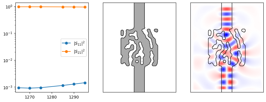
Now, we’ll plot the scattering parameters and the fields. We’ll define a plotting function so it can be reused below.

def plot_ceviche_component(component, params, response, aux):
    plt.figure(figsize=(11, 4))
    ax = plt.subplot(131)
    for i in range(response.s_parameters.shape[-1]):
        ax.semilogy(
            response.wavelengths_nm,
            onp.abs(response.s_parameters[:, 0, i]) ** 2,
            "o-",
            label="$|S_{" + f"{i + 1}1" + "}|^2$",
        )
    ax.legend()

    # Get the full structure, including waveguides extending away from the deisgn.
    density = component.ceviche_model.density(params.array)
    contours = measure.find_contours(density)

    ax = plt.subplot(132)
    im = ax.imshow(1 - density, cmap="gray")
    im.set_clim([-2, 1])
    for c in contours:
        plt.plot(c[:, 1], c[:, 0], "k", lw=1)
    ax.set_xticks([])
    ax.set_yticks([])

    ax = plt.subplot(133)
    fields = onp.real(aux["fields"][2, 0, :, :])
    im = ax.imshow(fields, cmap="bwr")
    im.set_clim([-onp.amax(onp.abs(fields)), onp.amax(onp.abs(fields))])
    for c in contours:
        plt.plot(c[:, 1], c[:, 0], "k", lw=1)
    ax.set_xticks([])
    ax.set_yticks([])


plot_ceviche_component(component, params, response, aux)