Meta-atom library

The meta-atom library challenge entails designing a library of sub-wavelength meta-atoms that impart a phase shift to normally-incident plane waves. The challenge targets three wavelengths: 450 nm, 550 nm, and 650 nm, and so a meta-lens built from the meta-atom library could be used for broadband visible light applications.

The challenge is based on “Dispersion-engineered metasurfaces reaching broadband 90% relative diffraction efficiency” by Chen et al., in which meta-atoms were found by a particle swarm approach and FDTD simulation.

Simulating existing designs

In this notebook we will evaluate a solution to the challenge from the invrs-gym paper.

from totypes import json_utils

import numpy as onp
import matplotlib.pyplot as plt
from skimage import measure

file = "241024_mfschubert_a522d59bd3da6f788398482bf559d58ef86530bf8ed491b602087d2d64ac6c86.json"

with open(f"../../../reference_designs/meta_atom_library/{file}", "r") as f:
    serialized = f.read()

params = json_utils.pytree_from_json(serialized)

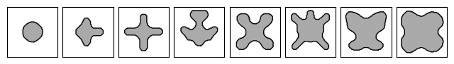
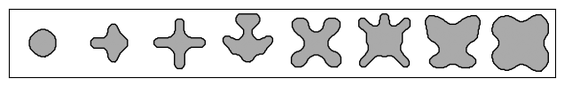
# Plot the eight meta-atoms.
_, axs = plt.subplots(1, 8, figsize=(8, 2))
for i, ax in enumerate(axs.flatten()):
    im = ax.imshow(1 - params["density"].array[i], cmap="gray")
    im.set_clim([-2, 1])
    for c in measure.find_contours(onp.array(params["density"].array[i])):
        ax.plot(c[:, 1], c[:, 0], "k", lw=1)
    ax.set_xticks([])
    ax.set_yticks([])
plt.subplots_adjust(hspace=0.1, wspace=0.1)

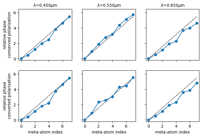
Figures 2a and 2b of Chen et al. plot the expected relative phase for the conserved and converted polarizations. We extracted the values from the figure, and replot them here. They will serve as a reference against which we compare the wavelength-dependent relative phase for the designs plotted above.

# Data from figs 2a and 2b of Chen et al.
expected_conserved = (
    (0.000, 0.451, 1.212, 1.985, 2.471, 3.843, 4.641, 5.489),  # 450 nm
    (0.000, 0.925, 1.898, 2.783, 3.195, 4.354, 5.140, 5.738),  # 550 nm
    (0.000, 0.501, 1.137, 1.910, 2.259, 3.693, 4.005, 4.641),  # 650 nm
)
expected_converted = (
    (0.000, 0.391, 1.137, 1.821, 2.194, 3.749, 4.632, 5.465),  # 450 nm
    (0.000, 0.900, 2.331, 2.567, 3.052, 4.308, 4.433, 5.540),  # 550 nm
    (0.000, 0.502, 1.137, 1.945, 2.306, 3.600, 3.861, 4.843),  # 650 nm    
)

_, axs = plt.subplots(2, 3, figsize=(8, 5))
for i, wavelength in enumerate([0.45, 0.55, 0.65]):
    axs[0, i].set_ylim([-0.2, 2 * onp.pi + 0.2])
    axs[1, i].set_ylim([-0.2, 2 * onp.pi + 0.2])
    axs[0, i].set_title(f"$\lambda$={wavelength:.3f}$\mu$m", fontsize=10)
    if i > 0:
        axs[0, i].set_yticklabels([])
        axs[1, i].set_yticklabels([])
    axs[0, i].set_xticklabels([])
    axs[1, i].set_xlabel("meta-atom index")

    axs[0, i].plot((0, 7), (0, 2 * onp.pi * 7 / 8), "k--", lw=1)
    axs[1, i].plot((0, 7), (0, 2 * onp.pi * 7 / 8), "k--", lw=1)

    axs[0, i].plot(expected_conserved[i], "o-")
    axs[1, i].plot(expected_converted[i], "o-")


axs[0, 0].set_ylabel("relative phase\nconserved polarization")
_ = axs[1, 0].set_ylabel("relative phase\nconverted polarization")

Now, we’ll simulate the above nanostructures and compute the phase imparted by each upon incident right-hand and left-hand circularly polarized light. We do this using the meta_atom_library challenge.

import jax.numpy as jnp
from invrs_gym.challenges import meta_atom_library
from invrs_gym.utils import transforms

challenge = meta_atom_library()
response, _ = challenge.component.response(params)

Extract the phase of the conserved and converted polarization components, and compare these to values taken from Chen et al. We also plot the transmission into the conserved and converted polarization modes.

def _relative_phase(t):
    t = onp.array(t)
    phase = onp.angle(t)
    phase = phase - phase[0, ...]
    offsets = onp.arange(-1, 2) * 2 * onp.pi
    for i in range(1, 8):
        target = i * onp.pi / 4
        for j in range(3):
            candidates = phase[i, j] + offsets
            idx = onp.argmin(onp.abs(target - candidates))
            phase[i, j] = candidates[idx]
    return phase

phase_conserved = _relative_phase(response.transmission_rhcp[:, :, 0])
phase_converted = _relative_phase(response.transmission_rhcp[:, :, 1])

_, axs = plt.subplots(3, 3, figsize=(8, 7))
for i, wavelength in enumerate([0.45, 0.55, 0.65]):
    axs[0, i].set_ylim([-0.2, 2 * onp.pi + 0.2])
    axs[1, i].set_ylim([-0.2, 2 * onp.pi + 0.2])
    axs[0, i].set_title(f"$\lambda$={wavelength:.3f}$\mu$m", fontsize=10)
    if i > 0:
        axs[0, i].set_yticklabels([])
        axs[1, i].set_yticklabels([])
    axs[0, i].set_xticklabels([])
    axs[1, i].set_xlabel("meta-atom index")

    axs[0, i].plot((0, 7), (0, 2 * onp.pi * 7 / 8), "k--", lw=1)
    axs[1, i].plot((0, 7), (0, 2 * onp.pi * 7 / 8), "k--", lw=1)

    axs[0, i].plot(expected_conserved[i], "o-", label="Chen et al.")
    axs[0, i].plot(phase_conserved[:, i], "o-", label="invrs-gym")
    axs[1, i].plot(expected_converted[i], "o-", label="Chen et al.")
    axs[1, i].plot(phase_converted[:, i], "o-", label="invrs-gym")

    axs[2, i].plot(onp.abs(response.transmission_rhcp[:, i, 0])**2, "C3", label="conserved")
    axs[2, i].plot(onp.abs(response.transmission_rhcp[:, i, 1])**2, "C4", label="converted")

axs[0, 0].legend()
axs[0, 0].set_ylabel("relative phase\nconserved polarization")
axs[1, 0].set_ylabel("relative phase\nconverted polarization")
axs[2, 2].legend()
_ = axs[2, 0].set_ylabel("transmission")

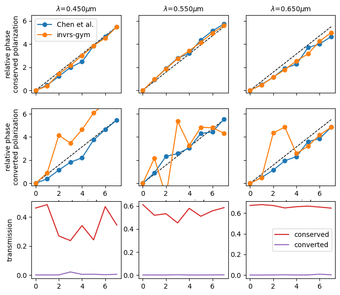
We see that the conserved polarization phase is quite linear, whereas the converted polarization is less so. This can be explained by differences in how the designs were optimized. In the paper by Chen et al., nanostructures were optimized to have linear phase profiles for both converted and conserved polarization, without directly considering the performance in e.g. a grating application. By contrast, the design from the invrs-gym paper was optimized using an objective function that considers the performance of a grating assembled from the meta-atoms, which effectively weights the phase objective with the transmission, so that overall grating performance is maximized.

Visualizing fields

Figure 1b of Chen et al. shows the phase of transmitted fields for a metagrating assembled from the meta-atom library plotted above. We’ll try to produce a similar figure, and start by assembling the meta-atoms into the supercell that comprises the metagrating.

import dataclasses

# Rotate and concatenate the meta-atoms into a supercell that is 8x1 in shape, matching the
# metagrating of Chen et al. Figure 1b.
density_tiled = dataclasses.replace(
    params["density"],
    array=jnp.concatenate(jnp.rot90(params["density"].array, axes=(1, 2)))[jnp.newaxis, :, :],
    fixed_void=None,
)

# Plot the supercell density.
density_tiled_plot = onp.array(density_tiled.array[0, ...].T)
_, ax = plt.subplots(1, 1, figsize=(8, 1))
im = ax.imshow(1 - density_tiled_plot, cmap="gray")
im.set_clim([-2, 1])
for c in measure.find_contours(onp.array(density_tiled_plot)):
    ax.plot(c[:, 1], c[:, 0], "k", lw=1)
ax.set_xticks([])
_ = ax.set_yticks([])

Next, use the simulate_library function from the library.component module. This function allows us to provide supercells for simulation, as well as batched individual meta-atoms.

import fmmax
from invrs_gym.challenges.library import component

# Since the supercell is larger, it requires more Fourier terms to ensure accuracy.
expansion = fmmax.generate_expansion(
    primitive_lattice_vectors=fmmax.LatticeVectors(
        u=fmmax.X * challenge.component.spec.pitch * 8,
        v=fmmax.Y * challenge.component.spec.pitch,
    ),
    approximate_num_terms=1200,
)

# Ensure that the `thickness_metasurface` attribute is a float, as required by
# the simulation method. In the default spec it is a bounded array, which is
# useful for optimization purposes.
spec = dataclasses.replace(challenge.component.spec, thickness_metasurface=0.6)

_, aux_fields = component.simulate_library(
    density=density_tiled,
    spec=spec,
    wavelength=jnp.asarray([0.45, 0.55, 0.65]),
    expansion=expansion,
    compute_fields=True,
)

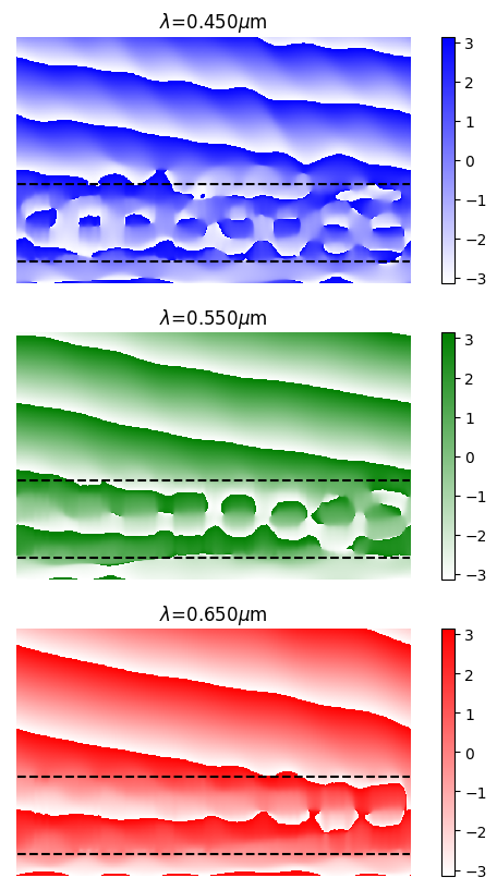
The phasefronts for fields in the metagrating are then plotted below.

ex, ey, ez = aux_fields["efield_xz"]

x, y, z = aux_fields["coordinates_xz"]
xplot, zplot = jnp.meshgrid(x, z, indexing="ij")
z_metasurface = challenge.component.spec.thickness_ambient
z_substrate = z_metasurface + params["thickness"].array

_, axs = plt.subplots(3, 1, figsize=(6, 10))

for i, (color, wavelength, ax) in enumerate(zip(["b", "g", "r"], [0.45, 0.55, 0.65], axs)):
    cmap = plt.cm.colors.LinearSegmentedColormap.from_list("b", ["w", color], N=256)
    im = ax.pcolormesh(xplot, zplot, jnp.angle(ex)[0, i, :, :, 0], cmap=cmap)
    ax.axis("equal")
    ax.set_ylim(ax.get_ylim()[::-1])
    ax.plot(x, jnp.full_like(x, z_metasurface), 'k--')
    ax.plot(x, jnp.full_like(x, z_substrate), 'k--')
    ax.axis(False)
    ax.set_title(f"$\lambda$={wavelength:.3f}$\mu$m")
    plt.colorbar(im)