Bayer sorter

The bayer sorter challenge involves the design of a Si3N4 metasurface to split light in a wavelength-dependent way, so that red, green, and blue light is predominantly collected in red, green, and blue subpixels in a sensor array. The challenge is based on Pixel-level Bayer-type colour router based on metasurfaces by Zou et al.

Simulating an existing design

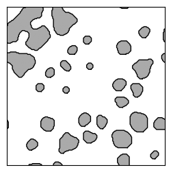
We’ll begin by loading, visualizing, and simulating the design from Supplementary Figure 2 of Zou et al.

import matplotlib.pyplot as plt
import numpy as onp
from skimage import measure

design = onp.genfromtxt("../../../reference_designs/bayer/zou.csv", delimiter=",")

plt.figure(figsize=(3, 3))
ax = plt.subplot(111)
im = plt.imshow(1 - design, cmap="gray")
im.set_clim([-2, 1])
ax.set_xticks([])
ax.set_yticks([])
for c in measure.find_contours(design):
    plt.plot(c[:, 1], c[:, 0], 'k', lw=1)

Next, create the bayer_sorter challenge, which enables us to simulate and evaluate a bayer sorter design.

The default simulation parameters are chosen to balance accuracy and simulation cost. For this notebook, we’ll override these with settings that yield more accurate results: more terms in the Fourier basis, and more wavelengths.

import dataclasses
import jax.numpy as jnp
from invrs_gym.challenges.bayer import challenge as bayer_challenge

challenge = bayer_challenge.bayer_sorter(
    sim_params=dataclasses.replace(
        bayer_challenge.BAYER_SIM_PARAMS,
        approximate_num_terms=1000,
        wavelength=jnp.arange(0.405, 0.7, 0.02),
    )
)

The params or optimization variables of the challenge include the metasurface pattern and also the metasurface thickness and metasurface-to-focal-plane separation. We’ll obtain default initial parameters from the challenge, and then overwrite the metasurface pattern with the array loaded and plotted above.

import jax

params = challenge.component.init(jax.random.PRNGKey(0))
assert params["density_metasurface"].shape == design.shape
params["density_metasurface"].array = design

Now, simulate the bayer sorter.

response, aux = challenge.component.response(params)

The response contains the transmission for normally-incident plane wave at the specified wavelengths for both x-polarized and y-polarized fields. The transmission is reported for four sub-pixels; the first is for red, the second and third for green, and the final is for blue.

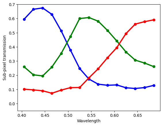
Plot the transmission into red, green, and blue subpixels

# Average the transmission over the two different incident polarizations.
transmission = onp.mean(response.transmission, axis=-2)

transmission_blue_pixel = transmission[:, 0]
transmission_green_pixel = transmission[:, 1] + transmission[:, 2]
transmission_red_pixel = transmission[:, 3]

plt.plot(response.wavelength, transmission_blue_pixel, "bo-", lw=3)
plt.plot(response.wavelength, transmission_green_pixel, "go-", lw=3)
plt.plot(response.wavelength, transmission_red_pixel, "ro-", lw=3)
plt.xlabel("Wavelength")
plt.ylabel("Sub-pixel transmission")
_ = plt.ylim(-0.05, 0.7)

The result is in very close agreement with Supplementary figure 7 of Zou et al.

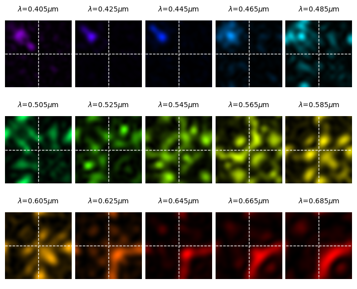
The transmission is computed by calculating the Poynting flux on the real-space grid at the focal plane, and summing within each sub-pixel quadrant. Since the fields are automatically computed during the course of a simulation, they are returned in aux.

Let’s plot the fields in the focal plane for each of the wavelengths.

import ccmaps

x, y = aux["coordinates_xy"]
x = jnp.squeeze(x, axis=0)
y = jnp.squeeze(y, axis=0)
ex, ey, ez = aux["efield_xy"]
intensity = jnp.abs(ex)**2 + jnp.abs(ey)**2 + jnp.abs(ez)**2
intensity = jnp.mean(intensity, axis=-1)  # Average over polarizations

fig, axs = plt.subplots(ncols=5, nrows=3, figsize=(9, 7))
axs = axs.flatten()
for i, wavelength in enumerate(response.wavelength):
    cmap = ccmaps.cmap_for_wavelength(wavelength_nm=wavelength * 1000)
    axs[i].pcolormesh(x, y, intensity[i, :, :], cmap=cmap)
    axs[i].set_ylim(axs[i].get_ylim()[::-1])
    axs[i].axis("equal")
    axs[i].axis(False)
    axs[i].plot([jnp.amin(x), jnp.amax(x)], [jnp.mean(y), jnp.mean(y)], "w--", lw=1)
    axs[i].plot([jnp.mean(x), jnp.mean(x)], [jnp.amin(y), jnp.amax(y)], "w--", lw=1)
    axs[i].set_title(f"$\lambda$={wavelength:.3f}$\mu$m", fontsize=10)

plt.subplots_adjust(wspace=0.05, hspace=0.25)