Metagrating#
The metagrating challenge entails designing a beam deflector that couples a normally-incident plane wave into one with a polar angle of 50 degrees. This problem was studied in “Validation and characterization of algorithms and software for photonics inverse design” by Chen et al.; the associated photonics-opt-testbed repo contains several example designs.
Simulating an existing design#
We’ll begin by loading, visualizing, and simulating designs from the photonics-opt-testbed repo.
import matplotlib.pyplot as plt
import numpy as onp
from skimage import measure
def load_design(name):
path = f"../../../reference_designs/metagrating/{name}.csv"
return onp.genfromtxt(path, delimiter=",")
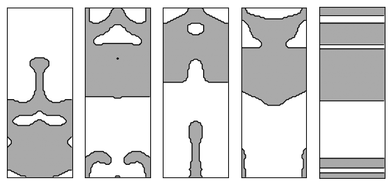
names = ["device1", "device2", "device3", "device4", "device5"]
designs = [load_design(name) for name in names]
plt.figure(figsize=(7, 4))
for i, design in enumerate(designs):
ax = plt.subplot(1, 5, i + 1)
im = ax.imshow(1 - design, cmap="gray")
im.set_clim([-2, 1])
contours = measure.find_contours(design)
for c in contours:
plt.plot(c[:, 1], c[:, 0], "k", lw=1)
ax.set_xticks([])
ax.set_yticks([])
Now, we’ll create a metagrating challenge, which provides everything we need to simulate and optimize the metagrating.
from invrs_gym import challenges

challenge = challenges.metagrating()
To simulate the metagrating, we need to provide a totypes.types.Density2DArray object to the challenge.component.params method. Obtain dummy parameters using component.init, and then overwrite the array attribute with the reference design that we want to simulate.
import dataclasses
import jax

dummy_params = challenge.component.init(jax.random.PRNGKey(0))
params = dataclasses.replace(dummy_params, array=load_design("device1"))

# Perform simulation using component response method.
response, aux = challenge.component.response(params)
The response contains the transmission and reflection efficiency into each diffraction order, and for TE- and TM-polarized cases. However, we only care about TM diffraction into the +1 order. Fortunately, the challenge has a metrics method that extracts this value.
metrics = challenge.metrics(response, params=params, aux=aux)
print(f"TM transmission into +1 order: {metrics['average_efficiency'] * 100:.1f}%")
TM transmission into +1 order: 95.6%
Now let’s take a look at the remaining designs.
for name in names:
    params = dataclasses.replace(dummy_params, array=load_design(name))
    response, aux = challenge.component.response(params)
    metrics = challenge.metrics(response, params=params, aux=aux)
    print(
        f"{name} TM transmission into +1 order: {metrics['average_efficiency'] * 100:.1f}%"
    )
device1 TM transmission into +1 order: 95.6%
device2 TM transmission into +1 order: 93.5%
device3 TM transmission into +1 order: 95.0%
device4 TM transmission into +1 order: 91.3%
device5 TM transmission into +1 order: 83.0%
These values are all very close to those reported in the photonics-opt-testbed, indicating that our simulation is converged.