Basic optimization example

In this notebook we’ll carry out basic unconstrained optimization of the metagrating challenge.

Start by creating a metagrating challenge, which provides everything we need to simulate and optimize the metagrating.

from invrs_gym import challenges

challenge = challenges.metagrating()

import jax

params = challenge.component.init(jax.random.PRNGKey(0))


def loss_fn(params):
    response, aux = challenge.component.response(params)
    loss = challenge.loss(response)
    metrics = challenge.metrics(response, params=params, aux=aux)
    efficiency = metrics["average_efficiency"]
    return loss, (response, efficiency)

To design the metagrating we’ll use the density_lbfgsb optimizer from the invrs-opt package. Initialize the optimizer state, and then define the step_fn which is called at each optimization step, and then simply call it repeatedly to obtain an optimized design.

import invrs_opt

opt = invrs_opt.density_lbfgsb(beta=4)
state = opt.init(params)  # Initialize optimizer state using the initial parameters.


@jax.jit
def step_fn(state):
    params = opt.params(state)
    (value, (_, efficiency)), grad = jax.value_and_grad(loss_fn, has_aux=True)(params)
    state = opt.update(grad=grad, value=value, params=params, state=state)
    return state, (params, efficiency)


# Call `step_fn` repeatedly to optimize, and store the results of each evaluation.
efficiencies = []
for _ in range(65):
    state, (params, efficiency) = step_fn(state)
    efficiencies.append(efficiency)

Now let’s visualize the trajectory of efficiency, and the final design.

import matplotlib.pyplot as plt
import numpy as onp
from skimage import measure

ax = plt.subplot(121)
ax.plot(onp.asarray(efficiencies) * 100)
ax.set_xlabel("Step")
ax.set_ylabel("Diffraction efficiency into +1 order (%)")

ax = plt.subplot(122)
im = ax.imshow(1 - params.array, cmap="gray")
im.set_clim([-2, 1])

contours = measure.find_contours(onp.asarray(params.array))
for c in contours:
    ax.plot(c[:, 1], c[:, 0], "k", lw=1)

ax.set_xticks([])
ax.set_yticks([])

print(f"Final efficiency: {efficiencies[-1] * 100:.1f}%")

Final efficiency: 96.2%

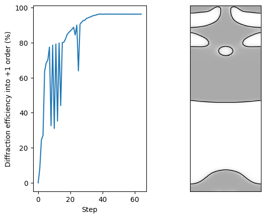
The final efficiency is around 90%, similar to the reference designs. However, note that the design is not binary, which is a limitation of the density_lbfgsb optimizer: it generally does not produce binary solutions. A different optimizer would be required to obtain binary designs.