Diffractive splitter

The diffractive splitter challenge entails designing a metasurface that evenly splits a normally-incident plane wave into a 7x7 array of beams. Light is incident from the ambient, with the substrate and the metasurface pattern being silicon oxide. The operating wavelength is 732.8 nm, and the unit cell pitch is 7.2 microns, corresponding to diffraction angles of ±15 degrees. The challenge is based on “Design and rigorous analysis of a non-paraxial diffractive beamsplitter” slide deck retrieved from the LightTrans web site.

Simulating an existing design

We’ll begin by loading, visualizing, and simulating several designs from the invrs-gym paper.

import matplotlib.pyplot as plt
import numpy as onp
from skimage import measure
from totypes import json_utils


def load_design(file):
    path = f"../../../reference_designs/diffractive_splitter/{file}"
    with open(path, "r") as f:
        serialized = f.read()
    return json_utils.pytree_from_json(serialized)

files = [
    "240413_mfschubert_40b6a186a2ad09fe4a4a9e8fbce60f5d38e39bf11f17102c0005612d8eb6df7b.json",
    "240413_mfschubert_ba86cdee2ff56eb6602b30bc0a87c995d6d4924cdd06fee0e949a9da3590d789.json",
    "240413_mfschubert_8d45bcf673d167db063065dab04b82a527a1e39e816e984c4ff3b4597ddc525a.json",
]

designs = [load_design(file) for file in files]

plt.figure(figsize=(8, 4))
for i, params in enumerate(designs):
    density = params["density"].array
    ax = plt.subplot(1, 3, i + 1)
    im = ax.imshow(1 - density, cmap="gray")
    im.set_clim([-2, 1])
    contours = measure.find_contours(density)
    for c in contours:
        plt.plot(c[:, 1], c[:, 0], "k", lw=1)
    ax.set_xticks([])
    ax.set_yticks([])

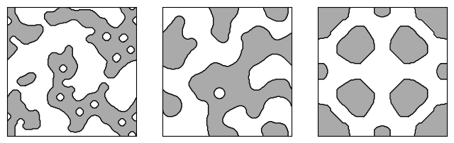
While several challenges involve only the design of two-dimensional patterns (with a Density2DArray being the optimization variable), the diffractive splitter degrees of freedom include both the metasurface pattern and several film thicknesses, in the form of a BoundedArray.

for key, value in designs[0].items():
    print(f"Variable {key}: {type(value)}")

Variable density: <class 'totypes.types.Density2DArray'>
Variable thickness_cap: <class 'totypes.types.BoundedArray'>
Variable thickness_grating: <class 'totypes.types.BoundedArray'>
Variable thickness_spacer: <class 'totypes.types.BoundedArray'>

Instantiate the challenge and simulate a design using the component.response method.

from invrs_gym.challenges.diffract import splitter_challenge

challenge = splitter_challenge.diffractive_splitter()

response, aux = challenge.component.response(params=designs[0])

Now let’s plot the diffraction efficiency for each order. We use the extract_orders_for_splitting function, and get the efficiency for a 9x9 array of beams (even though this design is for a 7x7 splitter). This will let us see how the diffraction efficiency drops off for orders beyond those targeted by the design.

plt.figure(figsize=(4, 3))

splitting = splitter_challenge.extract_orders_for_splitting(
    response.transmission_efficiency,
    response.expansion,
    splitting=(9, 9),
    polarization="TM",
)

ax = plt.subplot(111)
im = plt.imshow(splitting * 100, cmap="coolwarm")
ax.set_xticks(onp.arange(9))
ax.set_yticks(onp.arange(9))
ax.set_xticklabels(range(-4, 5))
ax.set_yticklabels(range(-4, 5))
plt.colorbar(im)
im.set_clim([0, onp.amax(splitting * 100)])
ax.set_title("device1\nDiffraction efficiency (%)")
_ = ax.set_ylim(ax.get_ylim()[::-1])

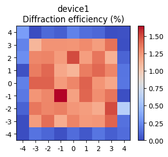
The device appears to have relatively good uniformity and efficiency. This can be quantified musing metrics compute using the challenge metrics method.

print("Solution 1 challenge metrics:")
for key, value in challenge.metrics(response, params=params, aux=aux).items():
    print(f"    {key} = {value:.4f}")

Solution 1 challenge metrics:

    binarization_degree = 1.0000
    total_efficiency = 0.6472
    average_efficiency = 0.0132
    min_efficiency = 0.0124
    zeroth_order_efficiency = 0.0132
    zeroth_order_error = -0.0026
    uniformity_error = 0.0602
    uniformity_error_without_zeroth_order = 0.0602

Let’s take a look at the remaining devices, which have larger feature sizes. We expect lower performance since the ability to exploit small features should contribute to high performance.

plt.figure(figsize=(8, 3))
for i, params in enumerate(designs[1:]):
    response, aux = challenge.component.response(params)

    splitting = splitter_challenge.extract_orders_for_splitting(
        response.transmission_efficiency,
        response.expansion,
        splitting=(9, 9),
        polarization="TM",
    )

    ax = plt.subplot(1, 2, i + 1)
    im = plt.imshow(splitting * 100, cmap="coolwarm")
    ax.set_xticks(onp.arange(9))
    ax.set_yticks(onp.arange(9))
    ax.set_xticklabels(range(-4, 5))
    ax.set_yticklabels(range(-4, 5))
    plt.colorbar(im)
    im.set_clim([0, onp.amax(splitting * 100)])
    ax.set_title(f"Solution {i + 2}\nDiffraction efficiency (%)")
    ax.set_ylim(ax.get_ylim()[::-1])

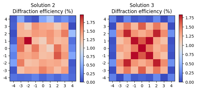
Observe that the symmetry in the layout of the third design results in symmetry in the diffraction efficiencies.